How a graph database turned scattered security alerts into connected attack stories, and what it took to make the visualization not look terrible.
In the first post I covered how Heimdall triages alerts using LLM sub-agents. But triage answers one question: is this alert real or noise? It doesn’t answer the harder question: if it’s real, how far did it go?
That’s the blast radius problem. A detection fires on a host. The process that triggered it also connected to an external IP. That IP resolved on two other hosts. One of those hosts had its own detection an hour earlier, involving the same user. Are these related? How do you even find out without spending 30 minutes clicking through different consoles?
The answer, at least for me, was to stop thinking about alerts as rows in a table and start thinking about them as a graph.
Why a Graph Database
Security data is inherently relational. A detection happens on a host, triggered by a process, run by a user, connecting to an IP, using a MITRE technique that belongs to a tactic. These aren’t flat records. They’re entities connected by relationships, and the interesting stuff lives in those connections.
Relational databases can model this with join tables, but the queries get ugly fast. “Find all detections that share a host, user, or IP with this detection” is a simple sentence but a painful SQL query with multiple self-joins. In Cypher (Memgraph’s query language), it’s almost readable:
MATCH (d:Detection {alertId: $alertId})-[:ON_HOST]->(h:Host)<-[:ON_HOST]-(d2:Detection)
WHERE d2 <> d
RETURN d2
I went with Memgraph over Neo4j for a practical reason: it runs entirely in memory, it’s lightweight enough to deploy as a single Docker container, and it speaks the Bolt protocol so the neo4j-driver npm package works out of the box. For a project that needs fast traversals on a relatively small graph (thousands of nodes, not millions), it’s a good fit.
The Data Model
The graph has seven node types and nine relationship types.
Nodes
- Detection – A security alert from CrowdStrike, Elastic, or AWS. Fields:
alertId,title,severity,timestamp - Host – An endpoint or server. Fields:
hostname,platform,OS - Process – A running process from the detection’s process tree. Fields:
filename,cmdline,sha256,pid - User – The user account involved. Fields:
username - IPAddress – An external IP associated with a host
- Technique – A MITRE ATT&CK technique. Fields:
techniqueId,name - Tactic – A MITRE ATT&CK tactic. Fields:
name
Relationships
ON_HOST– Detection to Host. Alert occurred on this endpointTRIGGERED_BY– Detection to Process. This process triggered the alertCHILD_OF– Process to Process. Parent/child process relationshipRUN_BY– Process to User. Process was executed by this userINVOLVES_USER– Detection to User. User associated with the detectionHAS_IP– Host to IPAddress. Host’s external IP addressUSES_TECHNIQUE– Detection to Technique. MITRE technique usedBELONGS_TO– Technique to Tactic. Technique falls under this tacticUSES_TACTIC– Detection to Tactic. Direct tactic association
The process tree is the most interesting part of the model. CrowdStrike detections include the triggering process plus its parent and grandparent. Heimdall creates a chain of Process nodes linked by CHILD_OF edges. The blast radius API extends this by fetching up to two additional levels of ancestry, so you can see the full lineage from the detection back to whatever kicked things off.
From Webhook to Graph
When a CrowdStrike alert arrives via webhook, Heimdall does two rounds of graph ingestion.
Round 1: Immediate. Right after the webhook payload is parsed and stored in SQLite, the raw alert data gets ingested into Memgraph. At this point the data is sparse. Maybe a hostname, a detection title, and basic MITRE mapping. But the node exists in the graph immediately.
Round 2: After enrichment. The Falcon API enrichment runs (the deterministic Phase 1 from the previous post), and the alert is re-ingested with the full process tree, network telemetry, external IPs, and proper technique/tactic mappings.
Before re-ingestion, Heimdall cleans up orphaned process nodes. If the original alert created three Process nodes and the enriched version has different ones (more detail, different command lines), the old process nodes get deleted if no other detection references them. This prevents the graph from accumulating stale data.
The ingestion itself is a single Cypher query built dynamically using MERGE statements. MERGE is important here because it creates a node only if it doesn’t already exist. Two detections on the same host don’t create two Host nodes. They both link to the same one. That’s what makes the graph work for correlation.
MERGE (d:Detection {alertId: $alertId})
SET d.title = $title, d.severity = $severity, ...

MERGE (h:Host {hostname: $hostname})
SET h.platform = $platform, ...

MERGE (d)-[:ON_HOST]->(h)
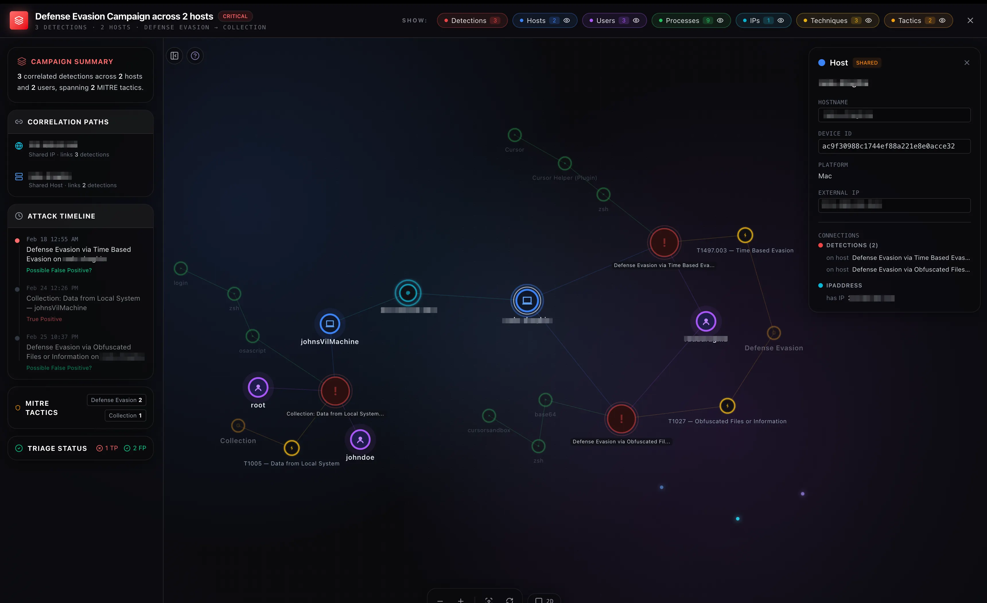
For processes, deduplication uses a combination of SHA256 hash and command line. The same binary with different arguments creates different Process nodes. The same binary with the same arguments reuses the existing node. This means if two detections involve the same base64 --decode invocation, they both connect to the same Process node, and that shared connection shows up in the graph.
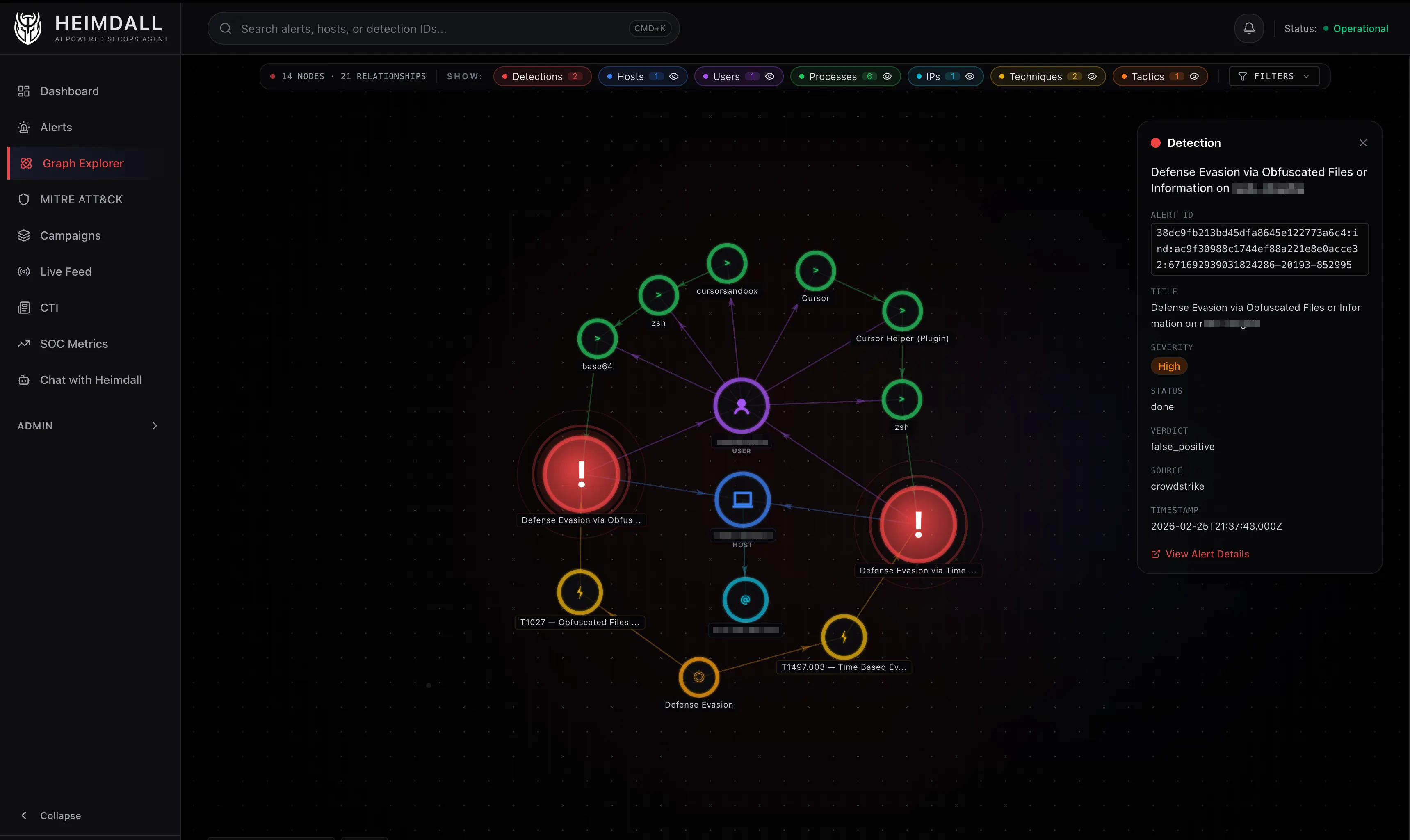
Blast Radius: How It Works
The blast radius query is the most complex piece of Cypher in the project. It runs in six steps, most of them in parallel.
Step 1: Find the central detection by alertId.
Step 2: Get everything directly connected to it (one hop). This gives you the host, user, processes, techniques, and tactics for the focal alert.
Step 3: Four parallel queries look for other detections that share an entity with the central detection:
- Shared host:
(d)-[:ON_HOST]->(h)<-[:ON_HOST]-(d2)whered2 != d - Shared user:
(d)-[:INVOLVES_USER]->(u)<-[:INVOLVES_USER]-(d2) - Shared IP:
(d)-[:ON_HOST]->(h)-[:HAS_IP]->(ip)<-[:HAS_IP]-(h2)<-[:ON_HOST]-(d2)whered2 != d - Shared technique:
(d)-[:USES_TECHNIQUE]->(t)<-[:USES_TECHNIQUE]-(d2)
Each query returns the bridging entity so the UI can show why two detections are related, not just that they are.
Related detections are filtered to a 48-hour window around the center alert. Without this, a workstation that accumulates unrelated false positives over weeks would show all of them in the blast radius. The 48-hour window keeps the focus on what was happening around the time of the detection – tight enough to filter temporal noise, wide enough to catch multi-stage activity that unfolds over a day or two.
Step 4: Get the entities of those related detections (second ring). Now you have the full picture: the focal detection, its entities, related detections, and their entities.
Step 5: Extend with extra hops. Technique to Tactic (BELONGS_TO), Host to IP (HAS_IP), and process ancestry chains (CHILD_OF up to two levels deep).
Step 6: Enrich with metadata from SQLite (severity, verdict, status, title) and return the whole thing as a flat list of nodes and links.
The result is a subgraph that answers: starting from this one alert, what else was happening nearby in time and topology?
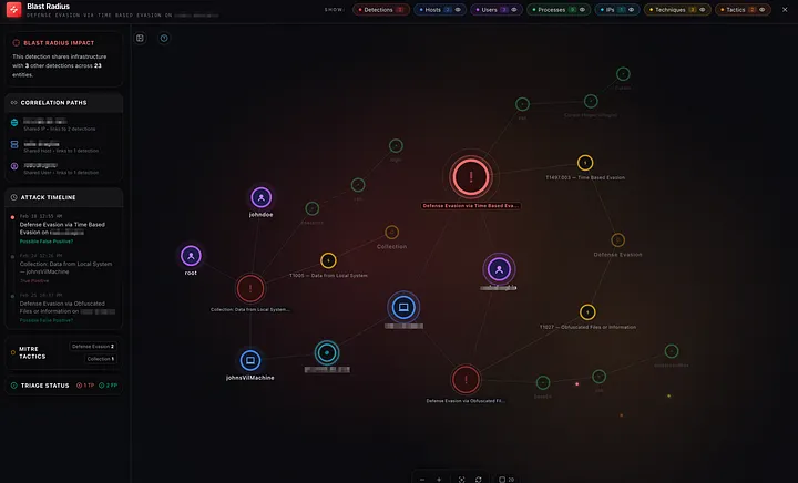
Campaign Detection with Union-Find
Campaigns are a layer above blast radius. While blast radius starts from one detection and expands outward, campaigns look at the entire graph and group detections that share entities.
The implementation uses Union-Find (also called disjoint set union), a data structure I honestly hadn’t used since university algorithms class.
Three Cypher queries run in parallel to find pairs of related detections:
- Same host: Two detections on the same host
- Same technique, different hosts: Two detections using the same MITRE technique but on different hosts. Same-host technique overlap is already covered by rule 1, so this specifically targets cross-host correlation
- Same IP, different hosts: Two detections whose hosts share an external IP but are different endpoints
Pairs are only formed between detections within 72 hours of each other. Without this, a corporate workstation that accumulates unrelated false positives over weeks would get lumped into a single “campaign.” Real coordinated attacks (lateral movement, persistence, exfiltration) typically unfold within hours to a few days, so 72 hours is wide enough to catch multi-stage activity but narrow enough to filter temporal noise.
const uf = new UnionFind();

for (const { a, b } of correlationPairs.filter(withinWindow)) {
  uf.union(a, b);
}

const campaigns = uf.components()
  .filter(group => group.length >= 2);
The campaign ID is a deterministic hash of the sorted alert IDs in the group, so it stays stable across refreshes as long as group membership doesn’t change.
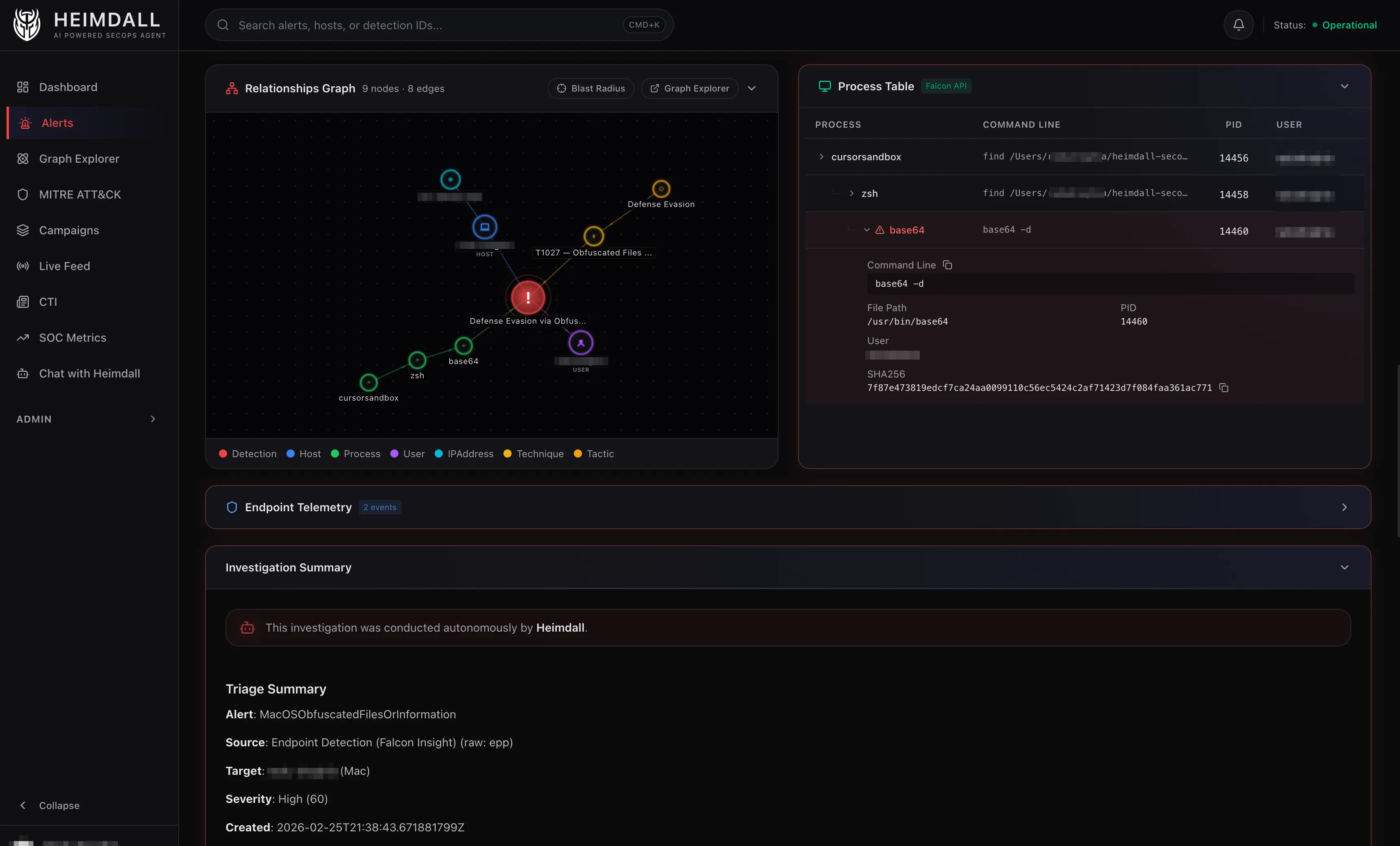
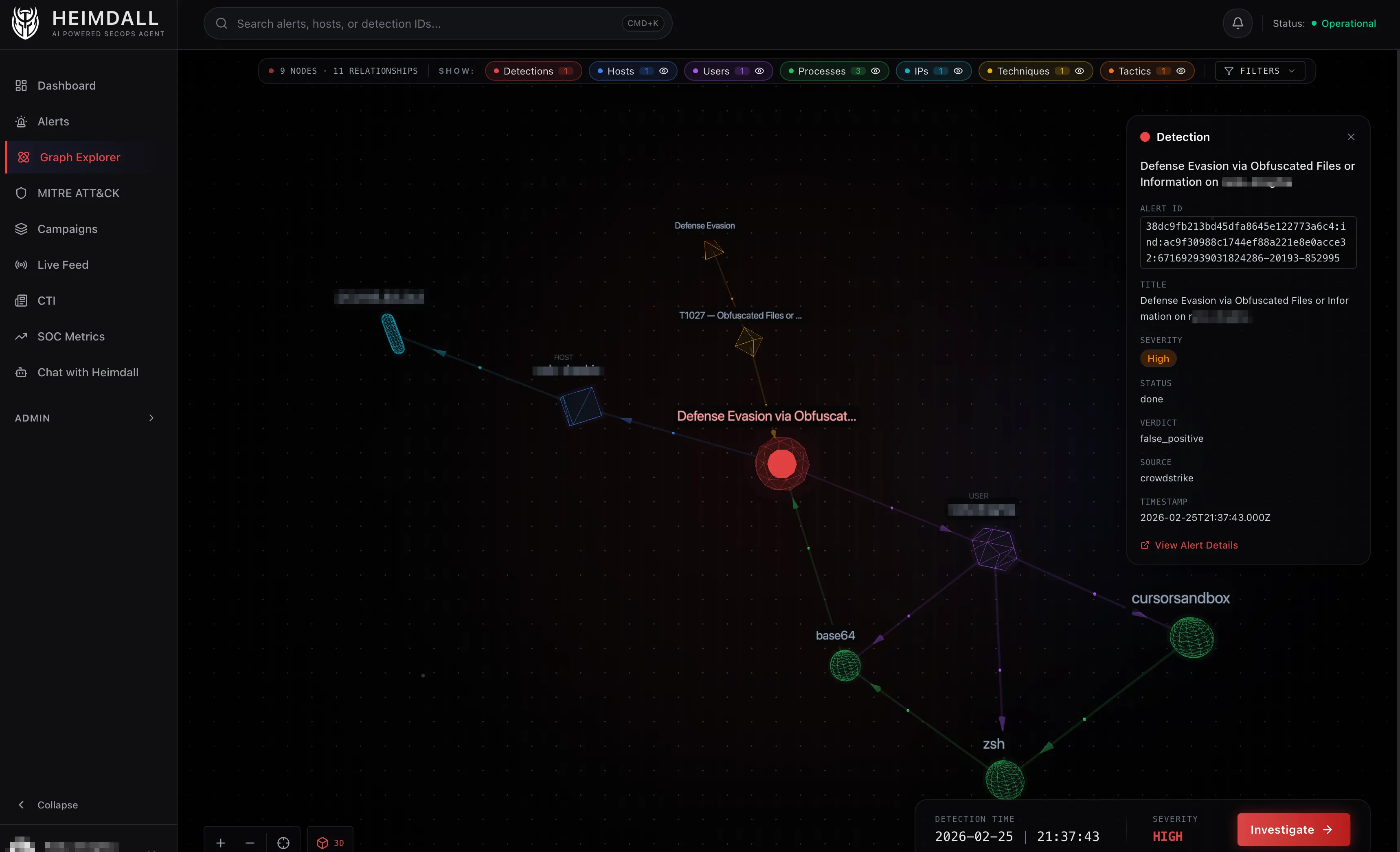
The Visualization
This is where I spent way more time than I expected.
The graph is rendered with react-force-graph-2d (and react-force-graph-3d for 3D mode). These libraries wrap a force-directed simulation where nodes repel each other via charge force, connected nodes attract via link force, and the whole thing settles into a layout that (in theory) puts related nodes close together.
The Initial Layout Problem
The default behavior of a force-directed graph is to start with all nodes at random positions and let the physics sort it out. For security graphs, this produces garbage. Process chain topologies collapse into a vertical line because the forces are symmetrical and there’s nothing to break the symmetry.
My first attempt involved tweaking physics parameters: stronger charge, more warmup ticks, scatter forces to break symmetry, and an automatic relayout after the simulation settled. It made the initial layout better but introduced jitter when interacting with the graph.
What actually worked was much simpler: seed the initial positions using a radial layout based on node type, then let the simulation fine-tune from there. Detections go in the inner ring, hosts and users in the middle ring, processes and techniques in the outer ring. If there’s a center node (blast radius mode), it sits at the origin.
The simulation still runs after seeding, but it starts from a reasonable position instead of chaos, so it converges quickly without the visual mess.
Making Drag Feel Right
The default force-directed graph behavior pins everything after the simulation settles. So when you drag a detection, its connected processes and hosts stay where they are. Links stretch like rubber bands but nothing follows. It looks terrible.
The fix was to let the simulation run during drags. When you grab a node:
- Nodes you’ve previously placed stay fixed (tracked in a
userPinnedRefset) - Everything else gets unpinned and the simulation reheats gently
- Connected nodes naturally follow via link forces while charge keeps them from overlapping
- When you drop the node, it gets pinned and the simulation cools down over 350ms while neighbours settle
This gives you the untangling behavior you’d expect. Drag a detection to the left and its connected processes and techniques drift along with it.
2D Rendering
The 2D graph uses canvas rendering with custom nodeCanvasObject callbacks. Each node type gets its own visual treatment:
| Node | Shape | Color |
|---|---|---|
| Detection | Circle with pulsing rings | Red |
| Host | Circle with server icon | Blue |
| Process | Small circle | Green |
| User | Circle with person icon | Purple |
| IPAddress | Circle | Cyan |
| Technique | Circle with lightning icon | Yellow |
| Tactic | Circle | Amber |
Links are color-coded by type and directional arrows show relationship direction.
3D Mode
The 3D view was mostly a fun experiment, but it turned out to be genuinely useful for large graphs where 2D gets too cluttered.
Each node type maps to a different Three.js geometry:
- Detection – Icosahedron with pulsating aura
- Host – Cube
- Process – Sphere
- User – Dodecahedron
- IPAddress – Torus
- Technique – Octahedron (holographic wireframe)
- Tactic – Tetrahedron (holographic wireframe)
All shapes use a “neon glass” aesthetic: dark core, colored wireframe overlay, and a transparent glow layer. Links have directional particle flow showing which way relationships point.
Lessons Learned
MERGE is your friend. The entire graph model relies on Memgraph’s MERGE statement to deduplicate entities. Two detections on the same host automatically share a Host node. Correlation emerges from the graph structure rather than being explicitly computed.
Small graphs need stronger forces. Most force-directed graph tutorials are calibrated for large networks. Security graphs are usually 10-50 nodes. At that scale, default charge and link forces barely separate anything. I ended up with charge strengths of -700 to -1200, much stronger than the typical -30 to -100 you see in examples.
Seed positions matter more than physics tuning. I spent days adjusting alpha decay, velocity decay, collision strength, and scatter forces. The single biggest improvement was providing a reasonable starting layout and letting the simulation refine from there. Good initial conditions beat good parameters.
Process dedup is tricky. Using (sha256, cmdline) as the MERGE key for processes mostly works, but there are edge cases. The same binary with slightly different arguments creates duplicate nodes. Still iterating on this.
What’s Next
This covers how the graph is built, queried, and rendered. The next post will get into the MCP integration layer: how the agent talks to CrowdStrike, CloudWatch, and VirusTotal through Model Context Protocol servers, and why tool filtering and budgets matter more than you’d think.